Look up values in a list of data Let's say that you want to look up an employee's phone extension by using ...
Look up values in a list of data
Let's say that you want to look up an employee's phone extension by using their badge number, or the correct rate of a commission for a sales amount. You look up data to quickly and efficiently find specific data in a list and to automatically verify that you are using correct data. After you look up the data, you can perform calculations or display results with the values returned. There are several ways to look up values in a list of data and to display the results.
What do you want to do?
-
Look up values vertically in a list by using an approximate match
-
Look up values vertically in a list of unknown size by using an exact match
-
Look up values horizontally in a list by using an exact match
-
Look up values horizontally in a list by using an approximate match
-
Create a lookup formula with the Lookup Wizard (Excel 2007 only)
Look up values vertically in a list by using an exact match
To do this task, you can use the VLOOKUP function, or a combination of the INDEX and MATCH functions.
VLOOKUP examples


For more information, see VLOOKUP function.
INDEX and MATCH examples
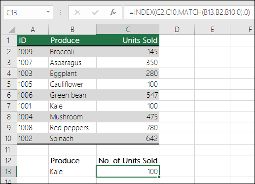
In simple English it means:
=INDEX(I want the return value from C2:C10, that will MATCH(Kale, which is somewhere in the B2:B10 array, where the return value is the first value corresponding to Kale))
The formula looks for the first value in C2:C10 that corresponds to Kale (in B7) and returns the value in C7 (100), which is the first value that matches Kale.
For more information, see INDEX function and MATCH function.
Look up values vertically in a list by using an approximate match
To do this, use the VLOOKUP function.
Important: Make sure the values in the first row have been sorted in an ascending order.
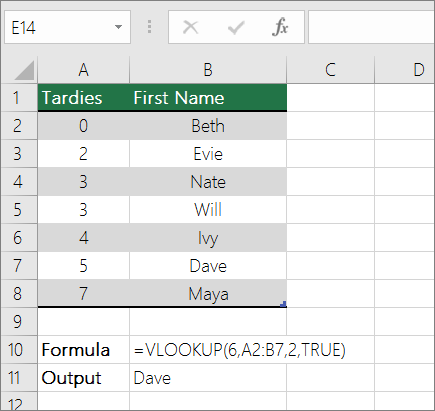
In the above example, VLOOKUP looks for the first name of the student who has 6 tardies in the A2:B7 range. There is no entry for 6 tardies in the table, so VLOOKUP looks for the next highest match lower than 6, and finds the value 5, associated to the first name Dave, and thus returns Dave.
For more information, see VLOOKUP function.
Look up values vertically in a list of unknown size by using an exact match
To do this task, use the OFFSET and MATCH functions.
Note: Use this approach when your data is in an external data range that you refresh each day. You know the price is in column B, but you don't know how many rows of data the server will return, and the first column isn't sorted alphabetically.
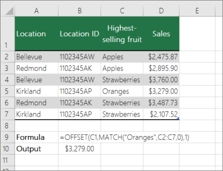
C1 is the upper left cells of the range (also called the starting cell).
MATCH("Oranges",C2:C7,0) looks for Oranges in the C2:C7 range. You should not include the starting cell in the range.
1 is the number of columns to the right of the starting cell where the return value should be from. In our example, the return value is from column D, Sales.
Look up values horizontally in a list by using an exact match
To do this task, use the HLOOKUP function. See an example below:
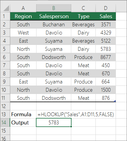
HLOOKUP looks up the Sales column, and returns the value from row 5 in the specified range.
For more information, see HLOOKUP function.
Look up values horizontally in a list by using an approximate match
To do this task, use the HLOOKUP function.
Important: Make sure the values in the first row have been sorted in an ascending order.
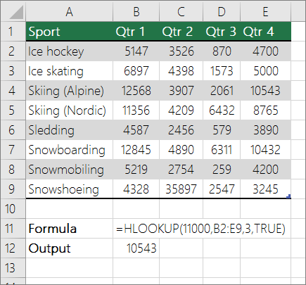
In the above example, HLOOKUP looks for the value 11000 in row 3 in the specified range. It does not find 11000 and hence looks for the next largest value less than 1100 and returns 10543.
For more information, see HLOOKUP function.
Create a lookup formula with the Lookup Wizard (Excel 2007 only)
Note: The Lookup Wizard add-in was discontinued in Excel 2010. This functionality has been replaced by the function wizard and the available Lookup and reference functions (reference).
In Excel 2007, the Lookup Wizard creates the lookup formula based on a worksheet data that has row and column labels. The Lookup Wizard helps you find other values in a row when you know the value in one column, and vice versa. The Lookup Wizard uses INDEX and MATCH in the formulas that it creates.
-
Click a cell in the range.
-
On the Formulas tab, in the Solutions group, click Lookup.
-
If the Lookup command is not available, then you need to load the Lookup Wizard add-in program.
How to load the Lookup Wizard Add-in program
-
Click the Microsoft Office Button
 , click Excel Options, and then click the Add-ins category.
 -
In the Manage box, click Excel Add-ins, and then click Go.
-
In the Add-Ins available dialog box, select the check box next to Lookup Wizard, and then click OK.
-
Follow the instructions in the wizard.


COMMENTS